Parameter Definitions

Choosing the model parameters that PEST can change to minimize the objective function is usually the first part of the setup.

An adjustable parameter can be described by its parameter type (e.g., hydraulic conductivity) and the assignment method (e.g., a certain geological formation).

• The Parameter type can be any time-constant material property of the FEFLOW model.
• The Assignment method can be based on zonally constant, pilot points and tied definitions.

The spatial definition of a adjustable parameter (zone or pilot point) can apply to any elemental selection that is stored in the FEFLOW model, to a FEFLOW layer or the entire model domain. FePEST also support the placement of pilot points in 3D.

Parametrization Methods

FePEST provides two options of model parametrization, which can be used during the model calibration:

Zonally constant

This is the most simple parametrization option, where one single parameter is assigned to a specific zone, region or volume.

 

Note that the choice for the zones already constitutes a kind of regularization (called structural regularization), that has the power to significantly influence the calibration process (in a good or bad way).

Pilot points

In the classical calibration approach, it is a common assumption that geologic formations have spatially constant parameter values. In reality, this is rarely true. The pilot-point method defines parameters as a spatially variable distribution. Therefore, instead of applying a homogeneous parameter value across a zone, varying values for the parameter are assigned at particular locations (the pilot points). Each pilot point represents an adjustable parameter within the PEST framework. Following the automatic adjustment at each PEST iteration, an interpolation method creates a continuous distribution of this parameter.

The resulting large number of parameters adds to the degrees of freedom in the inversion process. This will generally lead to a better fit to the measurement data. At the same time, it will increase the level of non-uniqueness and therefore better reproduce the uncertainty associated with the model predictions. Note that pilot-points are usually only used in combination with regularization to avoid overfitting.

 

 

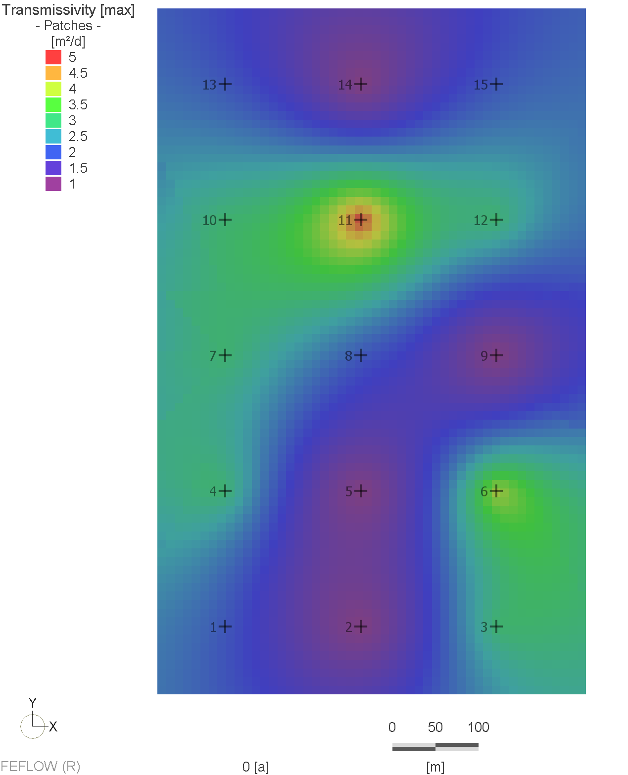
Distribution of hydraulic transmissivity, interpolated from a set of 15 pilot points.

 

Pilot points often lead to lower objective functions and better fits to measured data. However, the modeller should be aware of the risk of over-fitting the parameter field and should always check that the solution is plausible in terms of the conceptual model.

 

Further reading: PEST Groundwater Data Utilities, Part A, Chapter  5: Model Parameterization based on pilot-points.

 

Depending on the model projection (2D or 3D), FePEST provides a set of customized options for the assignment method via pilot points:

• Pilot points in 2D, all layers adjustable
• Pilot points in 2D, one layer adjustable, others tied
• Pilot points in 3D

 

The option "Apply as multiplier on existing values", available for parameters generated by means of the Pilot Points method, means the FEFLOW parameter values will not be replaced by the PEST parameter value before simulation, but rather the current FEFLOW parameter value will be multiplied by the PEST parameter value.

Option "Apply as as multiplier on existing values".

 

Further details about the parameter definitions is discussed in section Settings.