Monte Carlo Analysis

Monte Carlo analysis can be undertaken by FePEST to explore the uncertainty of a specific prediction or a set of predictions. From a groundwater modeller perspective, for example a prediction can be defined as the hydraulic heads in the model, inflows to a open-cast mine, concentrations at certain model areas, geothermal storage in the underground, etc.

The clear advantage of Monte Carlo analysis from a decision-maker point of view is the fact that we can learn the uncertainty of any prediction. Contrarily to other methods presented here (i.e. Predictive Analysis PEST mode), where uncertainty is only provided by one prediction at a time.

Predictive uncertainty analysis is accomplished by making predictions of interest with all parameter fields, and by then undertaking stochastic analysis of these predictions. The outcomes of this analysis include probability distributions (histograms) of individual predictions and/or group of predictions. From here we can learn about mean and variance of our predic­tions.

A definition of calibration-constrained Monte Carlo analysis stands for identi­fying multiple (i.e. several) model scenarios, which all of them maintains valid the assumption of calibration, i.e. minimum reduction of the measurement objective function. All these several model scenarios starts from a stochastic process (Monte Carlo) and after subsequent “adaptations”, they provide both an acceptable fit to the historical observations and reasonable parameter dis­tributions (i.e. regularized field).

The generation of parameter fields which respect calibration constraints is undertaken by combining the SVD-Assist as a mathematical regularization in PEST and the pre-calibration null-space projection of differences between stochastic parameter fields and the “calibrated” model.

Stochastic Parameter Generation

The start point of the analysis requires a model, which is considered to be “calibrated”. Such a stage can be achieved by running FePEST in the Estimation operation mode with any combination of regularization approaches and prior information.

Based on a Monte Carlo method, random parameters are generated with a mean value equal to the calibrated parameters. The prior information covari­ance matrix (Regularization - Tikhonov section in the Problem Settings dialog) and using a mean equal to the calibrated parameter field.

Null-Space Projection

The null-space projection is overtaken by the PEST Utility PNULPAR. The starting point of the null-space projection is a set of randomly-generated parameters and knowl­edge of the dimensionality of the problem.

Typically, the value of the calibrated parameters is considered as the mean value for the stochastic generation of the parameters. The number of dimen­sions of the calibrated solution space is approximately equal to the number of super parameters used by the SVD-Assist calibration.

During the operation of PNULPAR three task are carried out:

• Calculate the different between each parameter set and the calibrated parameters.

• This difference is subsequently projected onto the calibration null space

• The projected differenced is re-added to the calibrated parameter set.

The random parameter sets modified as described above do not strictly reflect a perfect calibrated model, because non-linearities in the problem. Therefore, adjustment of these parameters is required to validate the calibra­tion constraints. Such modifications take place through the alternations made to the calibration solution space (with an untouched null space).

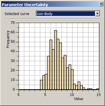
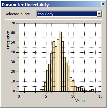
Parameter set (Conductivity) without null-space projection (left) and with null-space projection (right).

Figure above shows an example of randomly-generated parameters without (RANDPAR utility) and with (PNULPAR utility) projection onto the null space.

Readjustment of Parameters

In the previous steps, a set of “almost calibrated” parameters were gener­ated. In order to fully complete the calibration task for each parameter sam­ple, a series of calibration runs with PEST is undertaken. The SVD-Assist regularization in PEST is used here to adjust the parameters rapidly. This methodology will only run the model as many times as the number of super parameters (or dimensionality of the problem). Typically, after two iteration cycles of the PEST optimization, the calibration stage is achieved.

Outcome of Calibration-Constrained Monte Carlo

The final outcome of the calibration-constrained Monte Carlo provides a set model parameters, which all of them calibrate the model similarly. In addition we have tracked the evolution of a prediction (or several ones) and the evolu­tion of the objective function for all these models. These last two can be used to create histograms to understand explore the uncertainty of the modelling task.