PEST Algorithm

The fundamental methods applied by PEST during the calibration process are briefly described in the current section. This description below allows the reader to quickly understand their respective role in the overall workflow. The PEST documentation, to which specific references are provided, describes the methods in full detail.

The search algorithm used in PEST is the Gauss-Levenberg-Marquardt algorithm (GLMA). The central feature of the PEST engine is the GLMA search algorithm, that iteratively optimizes the model parameters to improve its fit to observed data and other objectives. The fit to the observations is hereby expressed through the Measurement Objective Function. In the simplest case, this will be the weighted sum of squares of the residuals between measurement and simulation results:

where (h^obs denotes an observation (typically from a field measurement), h^sim its related simulation result, and w the weight that has been applied to the measurement.

The observations hi are loaded from the FEFLOW model and the weights wi can be changed by the user within the FePEST user interface.

.

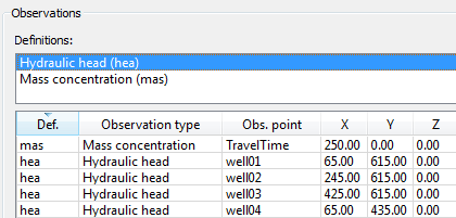
The objective function is defined through the observation definition in FePEST.

The GLMA changes the model parameters until a mini­mum objective function value is found. Running PEST, the user will observe two working steps per iteration:

• Derivative calculation: The parameters are changed incrementally. By repeating the model run for each parameter, and observing the resulting changes of observation values, the partial derivative for each pair of parameter and observation can be calculated by finite-difference approx­imation. These derivatives form the elements of the Jacobian matrix. The numerical effort to calculate the Jacobian matrix usually dominates the iteration. PEST has the option for switching from a 2, 3 and 5 point derivative calculation.

• The parameter values are adjusted aiming to reduce the objective func­tion. The direction and magnitude of the adjustment is expressed by the parameter upgrade vector. To identify the optimal direction of this vec­tor, the GLMA uses a combination of two strategies:

• While the objective function shows a predominantly linear behaviour, the method of gradient descent is applied. This method determines the parameter upgrade vector from the direction of steepest descent of the objective function. This can often be observed during the initial phase of the optimization.

• Objective-function nonlinearity is addressed via the Gauss-Newton method. This method computes a parameter upgrade vector based on the presumption of a quadratic behaviour of the objective function.

 

The two methods are not mutually exclusive: The GLMA interpolates between them, controlled by a scaling parameter named as the Marquardt-Lambda.

PEST dynamically updates lambda depending on the progress in reducing the objective function. The current lambda as displayed by FePEST during the PEST run is a good indicator for the current nonlinearity of the objective function.

• high lambda values (e.g., > 10) indicate linear behaviour (and predomi­nant use of the gradient descent method).

• small lambda values (e.g., < 2) indicate nonlinear behaviour (and predom­inant use of the Gauss-Newton method).

 

Figures below illustrate the development of the objective function and the Marquardt-Lambda during a typical PEST optimization. Gradient descent is used in the first iterations, indicated by higher lambda values. When the objective function approaches its (local) minimum, Lambda falls to near zero indicating almost exclusive use of the Gauss-Newton method

.

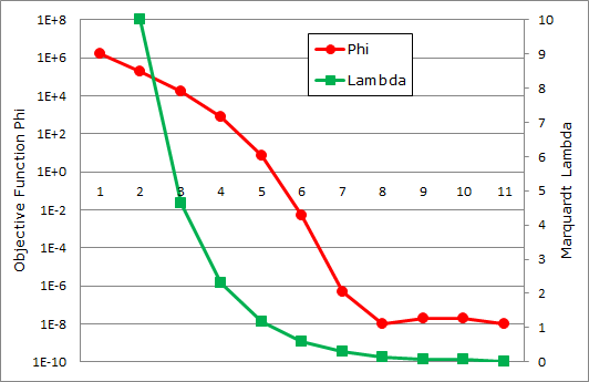
Development of the objective function and the Marquardt lambda during a PEST run.

.

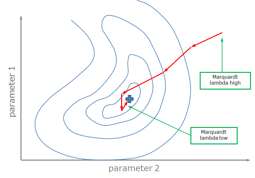
Schematic illustration of contours of the objective function and the path of the parameter upgrades vectors (after Doherty).

If successful, the GLMA will find a parameter set that constitutes a local min­imum of the defined objective function. This is an important restriction because multiple local minima might be present, and it is not guaranteed that the one found is also the global minimum.

It is therefore possible that different PEST runs result in different parameter sets if the iteration starts at different initial parameter values. These should therefore be chosen as close as possible to those values that are expected.

The modeller should also critically review the resulting parameter set and the model-to-measurement-misfit. Strong, but also very low departures indicate potential problems with the optimiza­tion.

 

PEST Manual (5th Ed.), Chapter 2.1: The Mathematics of PEST.

 

 

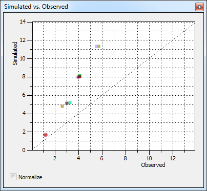
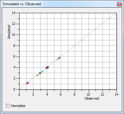
Scatter plot of simulated versus observed data before (top) and after (bot­tom) optimization.

Derivative Calculation

The calculation of derivatives is a fundamental element of the GLMA. The derivatives are calculated through numerical differentiation. Each param­eter is incrementally changed, and the model is run each time to calculate and record the resulting change of the model observations. The derivative of each parameter â observation relationship is then calculated through finite-difference techniques.

Correct calculation of derivatives is of critical importance to the optimization, as failure to it will lead to an unstable optimization procedure and PEST will not be able to lower the objective function.

 

Model instabilities are a frequent cause of PEST optimization failure!

 

 

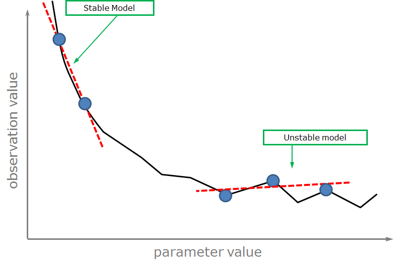
Schematic representation of a model response versus an input parameter change. Calculation of derivatives during stable (left) and unstable (right) model behaviour.

 

If the model is unstable, random noise dominates the physical change of the observation value. PEST tries to compensate with higher-order finite-difference methods.

Instabilities introduce noise to the observation, which is random and not related to the physical-based simulation result. If this noise - and not the incremental parameter change - dominates the obser­vation response, the direction of the upgrade vector becomes random itself and the optimization will fail.

Even though certain countermeasures are available, the modeller should always aim at maintaining maximum stability of the FEFLOW model. With PEST utility JACTEST, PEST provides a tool to check the integ­rity of the derivatives calculation for specified parameters.

 

PEST Manual (5th Ed.), Chapter 2.3: The Calculation of Deriva­tives.

Parameter Non-uniqueness

A typical challenge when history-matching (calibrating) an environmental model is the inherent non-uniqueness associated to the inverse solution. Usually many different parameter sets exist which are all compatible with the historical observation data.

Observation data is usually sparse and usually not sufficient to uniquely iden­tify more than just a few of the large number of model parameters that can be made adjustable. This has two consequences:

• Different calibrated parameter sets lead to different predictions. This makes it difficult to use a single model alone for decision-making.

• Some or many of the parameters will be insensitive to observations. The GLMA-based optimization process can become unstable under this con­dition, leading to long optimization run-times or even failure to optimise.

 

Regularization techniques can provide a defence against these issues. They restrict the parameter search to identifiable parameters, either by add­ing additional constraints to the parameters (Tik­honov Regularization) or separating identifiable parameters from non-identifiable parameters (Subspace Regularization). You can find more information about these methods in the section Regularization.